
Llama 2 Explained
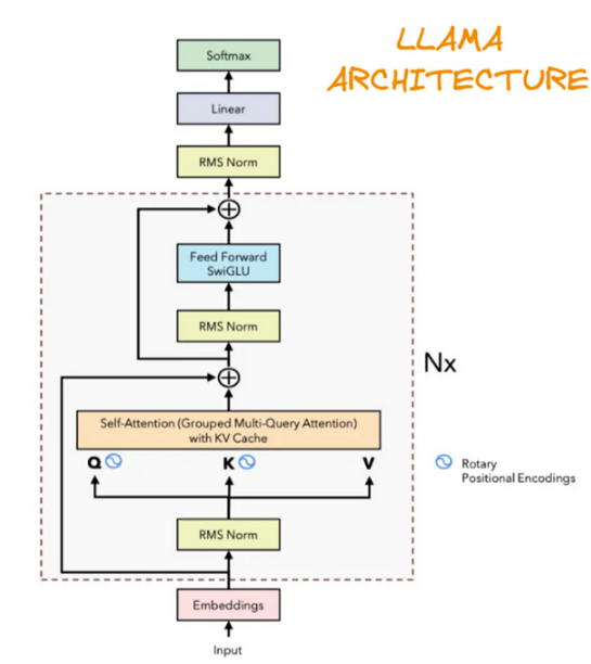
Meta's Llama 2 model represents a significant advancement in open-source large language models. In this deep dive, we'll explore the architecture, key innovations like Grouped Query Attention, KV Cache, and the training methodology that makes Llama 2 so powerful.
Llama 2 Architecture Overview
Llama 2 follows the decoder-only transformer architecture, similar to GPT models. It comes in three sizes: 7B, 13B, and 70B parameters. The architecture consists of the following components:
- Token Embeddings: Convert input tokens to vectors in a high-dimensional space
- Transformer Blocks: The core computational units (multiple layers)
- RMSNorm: Used for pre-normalization in each transformer block for improved training stability
- SwiGLU Activation: An improved activation function in the feed-forward networks
- Rotary Positional Embeddings (RoPE): Encodes position information directly in the attention computation
- Grouped-Query Attention (GQA): A key innovation for efficiency
The model processes text by first tokenizing it (breaking it into smaller units), embedding these tokens, passing them through multiple transformer blocks, and finally projecting to vocabulary probabilities.
Positional
Embedding
Root Mean Squared Normalization (RMSNorm)
Previously, LayerNorm was being used extensively for normalizing. It normalizes the layers rows-wise, which means it normalizes each feature independently. This allows model to amplify the scale of each feature or apply a translation to the feature according to the needs of the loss function.
LayerNorm can be mathematically represented as:
1class SimpleLayerNorm(nn.Module):
2    def __init__(self, normalized_shape: int, eps: float = 1e-5):
3        """
4        A simple implementation of Layer Normalization.
5
6        Args:
7            normalized_shape (int): the number of features in the last dimension to normalize over.
8            eps (float): small value to avoid division by zero.
9        """
10        super().__init__()
11        self.eps = eps
12        self.weight = nn.Parameter(torch.ones(normalized_shape))  # γ
13        self.bias = nn.Parameter(torch.zeros(normalized_shape))   # β
14
15    def forward(self, x: torch.Tensor) -> torch.Tensor:
16        """
17        Applies layer normalization to the input.
18
19        Args:
20            x (torch.Tensor): input tensor of shape (..., normalized_shape)
21
22        Returns:
23            torch.Tensor: normalized tensor of same shape as input
24        """
25        mean = x.mean(dim=-1, keepdim=True)
26        var = x.var(dim=-1, unbiased=False, keepdim=True)
27        x_norm = (x - mean) / torch.sqrt(var + self.eps)
28        return self.weight * x_norm + self.bias
But LayerNorm has its drawbacks:
- It can be computationally expensive for large models.
- It may not always lead to the best convergence properties during training.
- It can introduce noise in the gradients, especially in large models.
The authors of RMSNorm Paper believe that the recentering of the input is not needed.
Unlike LayerNorm, which normalizes each feature independently, RMSNorm normalizes the activations across the batch dimension. This can lead to faster convergence and improved model performance.
RMSNorm can be implemented as:
1class RMSNorm(nn.Module):
2    def __init__(self, dim: int, eps: float = 1e-6):
3        super().__init__()
4        self.eps = eps
5        self.weight = nn.Parameter(torch.ones(dim))
6
7    def _norm(self, x: torch.Tensor) -> torch.Tensor:
8        return x / torch.sqrt(x.pow(2).mean(-1, keepdim=True) + self.eps)
9
10    def forward(self, x: torch.Tensor) -> torch.Tensor:
11        return self.weight * self._norm(x)
Rotary Positional Embeddings (RoPE)
In transformer models, positional embeddings are crucial for capturing sequential information. Llama 2 uses Rotary Positional Embeddings (RoPE), which encode position information directly into the attention computation.
RoPE uses complex numbers to represent positions, allowing the model to learn relationships between tokens in a more flexible way. This is done by rotating the query and key vectors in the complex plane based on their positions.
Traditional positional embeddings add a fixed vector to the input tokens to encode their positions. This works well for short sequences but can be limiting for longer sequences. RoPE, on the other hand, encodes position information directly into the attention computation, allowing the model to handle longer sequences more effectively.
Grouped-Query Attention (GQA): The Efficiency Innovation
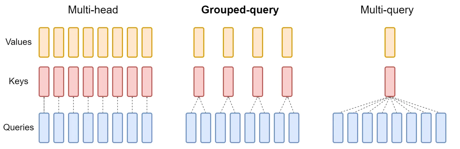
Comparison of MHA, MQA, and GQA attention mechanisms (Source: HuggingFace)
One of the most significant innovations in Llama 2 is Grouped-Query Attention (GQA). Traditional multi-head attention (MHA) has separate key (K), query (Q), and value (V) heads for each attention head. This creates a memory bottleneck during inference, especially for long sequences.
Here's a simplified implementation of GQA in PyTorch:
1class GroupedQueryAttention(nn.Module):
2    def __init__(self, args: Llama2Config) -> None:
3        super().__init__()
4
5        self.n_kv_heads = args.n_kv_heads if args.n_kv_heads is not None else args.n_heads
6        self.n_heads_q = args.n_heads
7        self.n_rep = self.n_heads_q // self.n_kv_heads
8
9        self.head_dim = args.dim // args.n_heads
10
11        self.wq = nn.Linear(args.dim, args.n_heads * self.head_dim, bias=False)
12        self.wk = nn.Linear(args.dim, self.n_kv_heads *
13                            self.head_dim, bias=False)
14        self.wv = nn.Linear(args.dim, self.n_kv_heads *
15                            self.head_dim, bias=False)
16        self.wo = nn.Linear(args.n_heads * self.head_dim, args.dim, bias=False)
17
18        self.register_buffer("cache_k", torch.zeros((args.max_batch_size, args.max_seq_len, self.n_kv_heads, self.head_dim)), persistent=False)
19        self.register_buffer("cache_v", torch.zeros((args.max_batch_size, args.max_seq_len, self.n_kv_heads, self.head_dim)), persistent=False)
20
21    def forward(self, x: torch.Tensor, start_pos: int, freqs_complex: torch.Tensor) -> torch.Tensor:
22        batch_size, seq_len, _ = x.shape
23
24        xq = self.wq(x)
25        xk = self.wk(x)
26        xv = self.wv(x)
27
28        xq = xq.view(batch_size, seq_len, self.n_heads_q, self.head_dim)
29        xk = xk.view(batch_size, seq_len, self.n_kv_heads, self.head_dim)
30        xv = xv.view(batch_size, seq_len, self.n_kv_heads, self.head_dim)
31
32        xq = apply_rotary_embedding(xq, freqs_complex, x.device)
33        xk = apply_rotary_embedding(xk, freqs_complex, x.device)
34        xv = apply_rotary_embedding(xv, freqs_complex, x.device)
35
36        self.cache_k[:batch_size, start_pos:start_pos + seq_len] = xk
37        self.cache_v[:batch_size, start_pos:start_pos + seq_len] = xv
38
39        keys = self.cache_k[:batch_size, :start_pos + seq_len]
40        values = self.cache_v[:batch_size, :start_pos + seq_len]
41
42        keys = repeat_kv(keys, self.n_rep)
43        values = repeat_kv(values, self.n_rep)
44
45        xq = xq.transpose(1, 2)
46        keys = keys.transpose(1, 2)
47        values = values.transpose(1, 2)
48
49        scores = torch.matmul(
50            xq, keys.transpose(-2, -1)) / math.sqrt(self.head_dim)
51        attn_len = keys.size(2)
52        mask = torch.triu(
53            torch.full((seq_len, attn_len), float('-inf'), device=x.device),
54            diagonal=1
55        )
56        scores = scores + mask
57        scores = F.softmax(scores.float(), dim=-1).type_as(xq)
58
59        output = torch.matmul(scores, values)
60        output = (output.transpose(1, 2).contiguous().view(
61            batch_size, seq_len, -1))
62
63 return self.wo(output)KV Cache: Accelerating Generation
When generating text, language models process one token at a time. For each new token, they would need to recompute the key (K) and value (V) vectors for all previous tokens. The KV cache optimization stores these vectors after they've been computed once, making generation much faster.
Here's a simplified implementation of KV caching:
1def generate_with_kv_cache(model, input_ids, max_length):
2    batch_size = input_ids.shape[0]
3
4    # Initialize KV cache (for each layer in the model)
5    num_layers = len(model.layers)
6    past_key_values = [None] * num_layers
7
8    # Generate tokens one by one
9    for i in range(max_length):
10        # If first iteration, process the whole input
11        # Otherwise, only process the last generated token
12        if i == 0:
13            current_input = input_ids
14        else:
15            current_input = next_token.unsqueeze(1)
16
17        # Forward pass with KV cache
18        outputs = model(
19            current_input,
20            past_key_values=past_key_values,
21            use_cache=True
22        )
23
24        logits = outputs.logits
25        next_token_logits = logits[:, -1, :]
26
27        # Sample next token
28        next_token = torch.argmax(next_token_logits, dim=-1)
29
30        # Update input_ids with generated token
31        input_ids = torch.cat([input_ids, next_token.unsqueeze(-1)], dim=-1)
32
33        # Update KV cache for next iteration
34        past_key_values = outputs.past_key_values
35
36    return input_ids
The SwiGLU Activation Function
Llama 2 uses the SwiGLU activation function in its feed-forward networks. SwiGLU is a combination of the Swish activation function and the Gated Linear Unit (GLU).
SwiGLU can be mathematically represented as:
1def swiglu(x, w1, w2):
2    return x * torch.sigmoid(torch.matmul(x, w1) + torch.matmul(x, w2))
Training Details: How Llama 2 Was Built
Llama 2 was trained using a massive dataset and sophisticated training methodology:
Pretraining
- Dataset: 2 trillion tokens from publicly available sources
- Tokenizer: BPE tokenizer with a vocabulary of 32K tokens
- Optimization: AdamW optimizer with cosine learning rate schedule
- Context Length: Trained on sequences of up to 4,096 tokens
- Compute: Trained on thousands of GPUs for millions of GPU-hours
Fine-tuning for Chat
Llama 2-Chat models underwent an extensive fine-tuning process:
- Supervised Fine-Tuning (SFT): Initial fine-tuning on human-generated demonstration data to follow human instructions
- Reinforcement Learning from Human Feedback (RLHF):
- Created a reward model from human preference data
- Used Proximal Policy Optimization (PPO) to optimize the model based on the reward function
- Red Teaming and Safety: Extensive testing and iteration to reduce harmful outputs and improve helpfulness
Architectural Details
Let's look at the specific architecture details for each model size:
| Parameter | Llama 2 7B | Llama 2 13B | Llama 2 70B |
|---|---|---|---|
| Hidden Size | 4,096 | 4,096 | 4,096 |
| Intermediate Size | 11,008 | 11,008 | 11,008 |
| Num Attention Heads | 32 | 40 | 64 |
| Num KV Heads (GQA) | 32 | 40 | 8 |
| Num Layers | 32 | 40 | 80 |
| RMS Norm Eps | 1e-6 | 1e-6 | 1e-6 |
Notice how the 70B model uses only 8 KV heads despite having 64 attention heads, demonstrating the efficiency gains from Grouped-Query Attention.
Performance Improvements from Llama 1 to Llama 2
Llama 2 introduced several improvements over its predecessor:
- 2× More Training Data: More tokens during pretraining
- Longer Context Length: 4K tokens vs 2K in Llama 1
- Grouped-Query Attention: For improved inference efficiency
- Enhanced RLHF: More sophisticated alignment techniques
- Improved Safety: More robust against generating harmful content
These improvements collectively led to significant performance gains across various benchmarks, with Llama 2 outperforming similarly sized open-source models and approaching the capabilities of proprietary models in many cases.
Limitations and Challenges
Despite its impressive capabilities, Llama 2 still faces several challenges:
- Hallucinations: Like all large language models, Llama 2 can generate incorrect information confidently
- Limited Context Window: While improved to 4K tokens, still limited compared to some newer models with 8K-32K context lengths
- Training Data Cutoff: Knowledge limited to data available during training
- Bias and Fairness: May reflect biases present in the training data
Conclusion
Llama 2 represents a significant advancement in open-source large language models. Its innovative architecture, particularly the Grouped-Query Attention mechanism, strikes an excellent balance between computational efficiency and model quality. The KV cache optimization further enhances its performance during text generation.
The meticulous training methodology, combining massive-scale pretraining with sophisticated fine-tuning approaches, has produced a model that can serve as a foundation for numerous applications. As open-source models continue to evolve, Llama 2's architectural innovations will likely influence future developments in the field.
References:
If this resonated, pass it along.