March 24, 2025·20 min read

Attention and the versions of it: Layer by Layer

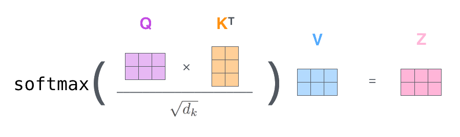
Attention MechanismTransformersSelf-AttentionSDPADeep LearningMachine LearningFlash AttentionSliding Window AttentionInfini-AttentionGrouped Query Attention

In the last blog, we talked about the Attention Mechanism and how it revolutionized the field of Natural Language Processing. But the vanilla Attention Mechanism has its limitations. In this blog, we will discuss the different versions of the Attention Mechanism and how they overcome these limitations.

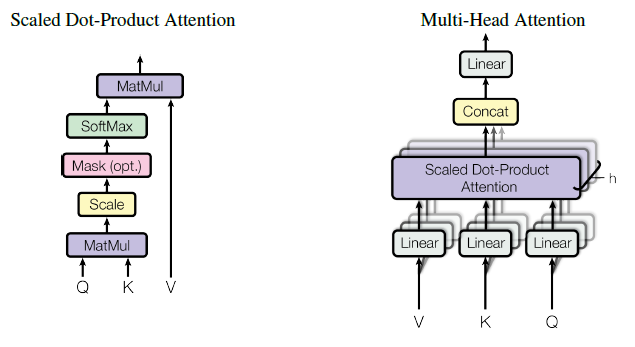
SDPA and Multi - Head Attention

Here are some of the attention types mentioned in my last blog:

Self Attention
Bidirectional Attention
Multi-Query Attention
Grouped Query Attention
Infini-Attention
Sliding Window Attention
Flash Attention

Each of these attention types has its own advantages and disadvantages. The choice of attention type depends on the problem at hand and the computational resources available. Let's discuss some of the attention types in detail.

I have written explanations of each line of the code for better understanding. If you wish to skip the explanation, you may not open the expanders.

1. Self Attention

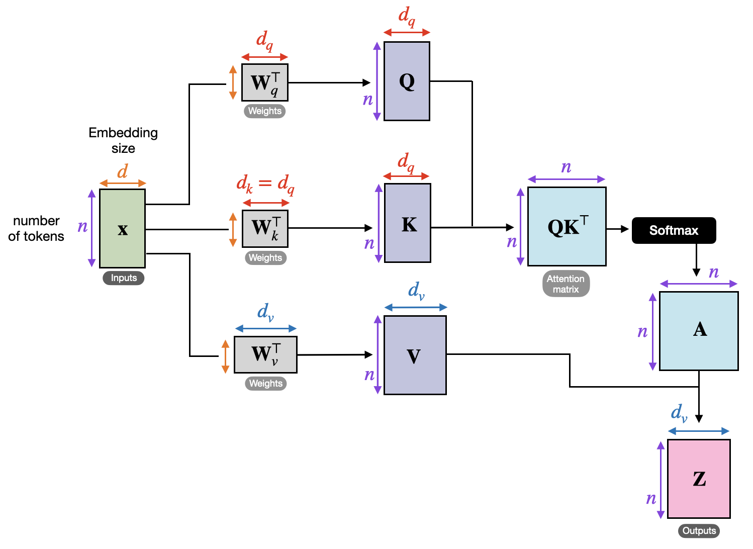
Self Attention

Self-Attention is the bread and butter of many modern NLP models. In this mechanism, every token in a sentence can interact with every other token. It’s like a networking event where everyone gets to chat with everyone else!

Power Points & Problems

Power: Captures global dependencies.
Problem: Time complexity being O(n²) makes it computationally expensive for long sequences.

Code Example: Self-Attention Class

1import torch
2import torch.nn as nn
3from torch.nn import functional as F
4
5
6class SelfAttention(nn.Module):
7    """One head of self-attention."""
8
9    def __init__(self, n_embd, head_size, block_size, dropout):
10        super().__init__()
11        self.key = nn.Linear(n_embd, head_size, bias=False)
12        self.query = nn.Linear(n_embd, head_size, bias=False)
13        self.value = nn.Linear(n_embd, head_size, bias=False)
14        self.register_buffer('tril', torch.tril(torch.ones(block_size, block_size)))
15        self.dropout = nn.Dropout(dropout)
16
17    def forward(self, x):
18        B, T, C = x.shape
19        k = self.key(x)
20        q = self.query(x)
21        wei = q @ k.transpose(-2, -1) * k.shape[-1] ** -0.5
22        wei = wei.masked_fill(self.tril[:T, :T] == 0, float('-inf'))
23        wei = F.softmax(wei, dim=-1)
24        wei = self.dropout(wei)
25        v = self.value(x)
26        out = wei @ v
27        return out

Explanation

1. Extracting Dimensions

18B, T, C = x.shape

What it does: This line unpacks the shape of the input tensor x into three variables:

- B: Batch size (how many samples are processed simultaneously).

- T: Sequence length (number of tokens or time steps).

- C: Embedding dimension (the size of the vector representation for each token).

Why it's important: Knowing these dimensions is crucial for subsequent tensor operations. Think of it as checking the ingredients before you bake a cake.

2. Computing Keys

19k = self.key(x)

What it does: Applies a linear transformation to the input x using the self.key layer, which is a nn.Linear without bias.

Why it's important: This projects the input data into the “key” space, producing a new tensor k that holds key vectors for each token. These keys will later be used to calculate similarity with queries.

3. Computing Queries

20q = self.query(x)

What it does: Similar to the previous step, this line applies a different linear transformation using the self.query layer to compute query vectors from the input.

Why it's important: The query vectors q represent what each token is looking for in the other tokens, kind of like a detective asking, "Who here is important for me to pay attention to?"

4. Calculating Scaled Dot-Product Attention Scores

21wei = q @ k.transpose(-2, -1) * k.shape[-1] ** -0.5

What it does:

- Matrix Multiplication (q @ k.transpose(-2, -1)): Multiplies the query tensor q with the transposed key tensor k. This computes dot products between queries and keys, resulting in a tensor of attention scores. The transposition ensures the multiplication aligns the embedding dimensions correctly.

- Scaling (* k.shape[-1] ** -0.5): Scales the result by the inverse square root of the key dimension (i.e., 1/sqrt(d_k)). This helps keep the gradients in a healthy range, especially when the dimensionality is large.

Why it's important: This line is the heart of the self-attention mechanism, determining how much attention each token should pay to every other token. Without the scaling factor, the dot products could become too large and lead to extremely small gradients after the softmax, which would be a training nightmare.

5. Applying the Causal Mask

23wei = wei.masked_fill(self.tril[:T, :T] == 0, float('-inf'))

What it does:

- Masking: Uses the lower-triangular matrix self.tril to mask out (i.e., ignore) the upper triangular part of the attention scores.

- masked_fill: Replaces the masked (future) positions with negative infinity (-inf), instructing the softmax to assign almost zero probability to these positions.

Why it's important: In autoregressive tasks like language modeling, you shouldn’t peek into future tokens. This mask enforces causality, ensuring that each token can only attend to itself and previous tokens.

6. Applying Softmax

24wei = F.softmax(wei, dim=-1)

What it does: Applies the softmax function along the last dimension of the tensor, converting the raw attention scores into a probability distribution.

Why it's important: Softmax ensures that the attention weights sum up to 1, effectively normalizing the “importance” of each token relative to every other token. It’s like converting raw exam scores into percentage grades.

7. Applying Dropout

25wei = self.dropout(wei)

What it does: Randomly zeroes some elements in the attention weights tensor based on the dropout probability provided.

Why it's important: Dropout is a regularization technique that helps prevent overfitting by ensuring the model doesn't become too reliant on any one set of weights. It’s like taking a quick break during a marathon to avoid burnout.

8. Computing Values

26v = self.value(x)

What it does: Applies another linear transformation to the input x using the self.value layer to compute the value vectors.

Why it's important: The value vectors v contain the information that will be combined based on the computed attention weights. They represent what information is being passed along to the next layers.

9. Producing the Final Output

27out = wei @ v

What it does: Multiplies the attention weights wei with the value vectors v, resulting in a weighted sum that aggregates the values based on their corresponding attention probabilities.

Why it's important: This is where the magic of self-attention happens. Each token’s final representation is a blend of the value vectors of all tokens, weighted by how much attention they deserve, like a committee vote where every token’s “voice” is considered.

Applications: Self-Attention is used in models like Transformer and GPT-3.

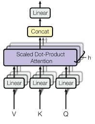
Multi Head Attention

This is the implementation of the single head of the self-attention mechanism that was given in the "Attention is All You Need" paper. The same paper also mentions that when multiple heads are used, we get performance improvements. This is because each head can learn different aspects of the data. This is where the Multi-Head Attention comes into play. Multi head attention is the same as self attention but with multiple parallel heads.

2. Bidirectional Attention

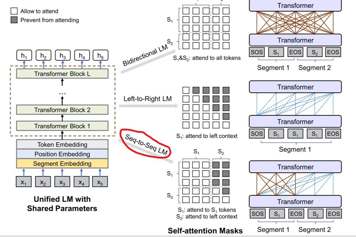
Bidirectional Attention difference with Self Attention

Bidirectional Attention allows tokens to look both left and right. Imagine being at a party where you’re not just scanning the room to your left—you’re scanning every corner. This method is especially useful for capturing context from both directions.

Power Points & Problems

Enhanced context understanding by attending to both past and future tokens.
Problem: Can introduce noise from irrelevant future context if not handled properly.

Code Example: Bidirectional Attention Class

1class BidirectionalAttention(nn.Module):
2    def __init__(self, embed_size):
3        super(BidirectionalAttention, self).__init__()
4        self.W_q = nn.Linear(embed_size, embed_size)
5        self.W_k = nn.Linear(embed_size, embed_size)
6        self.W_v = nn.Linear(embed_size, embed_size)
7    
8    def forward(self, x):
9        Q = self.W_q(x)
10        K = self.W_k(x)
11        V = self.W_v(x)
12        scores = torch.matmul(Q, K.transpose(-2, -1)) / math.sqrt(x.size(-1))
13        attention = torch.softmax(scores, dim=-1)
14        return torch.matmul(attention, V)

Explanation

1. Computing Query, Key, and Value Matrices

9Q = self.W_q(x)

10K = self.W_k(x)

11V = self.W_v(x)

What it does: The input tensor x is linearly transformed using three separate weight matrices: W_q, W_k, and W_v. These represent the queries, keys, and values, respectively.

Why it's important: This transformation projects the input into different spaces, which allows the model to determine attention scores based on the relationships between queries and keys.

2. Computing Attention Scores

12scores = torch.matmul(Q, K.transpose(-2, -1)) / math.sqrt(x.size(-1))

What it does:

Dot Product: The query matrix Q is multiplied with the transposed key matrix K, producing a similarity score for each pair of elements.
Scaling: The scores are divided by the square root of the embedding size. This prevents large values from dominating the softmax operation later, ensuring more stable gradients.

Why it's important: The attention scores determine how much focus each token should place on every other token.

3. Applying Softmax to Obtain Attention Weights

13attention = torch.softmax(scores, dim=-1)

What it does: Applies the softmax function along the last dimension, normalizing the scores into probabilities that sum to 1.

Why it's important: This converts raw attention scores into meaningful weights, determining how much each token contributes to the final representation.

4. Computing the Final Output

14return torch.matmul(attention, V)

What it does: The computed attention weights are multiplied by the value matrix V, generating a weighted sum of values.

Why it's important: This step produces the final representation of each token, considering information from all other tokens according to their computed importance.

Applications: Bidirectional Attention is used in models like BERT and T5.

3. Multi - Query Attention

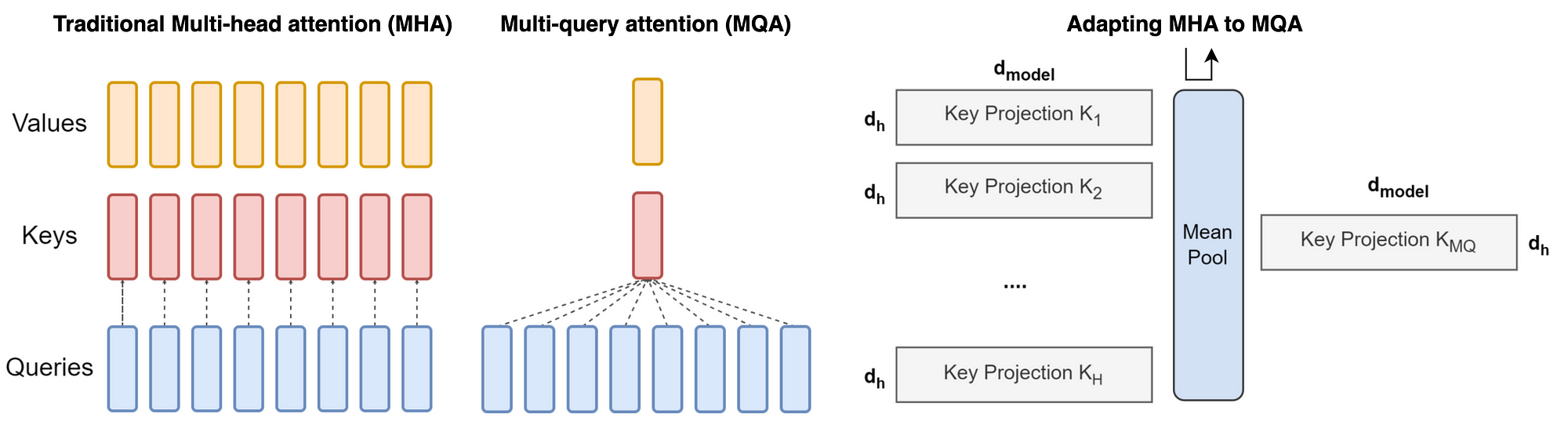
Multi Query Attention

Multi-Query Attention streamlines computation by sharing keys and values across heads, while still allowing separate queries. It’s like ordering one giant pizza and letting everyone take a slice instead of making multiple orders efficient, yet flexible.

Power Points & Problems

Reduces computation by sharing key and value matrices.
Problem: Can lead to less diversity in attention patterns across heads.

Code Example: Multi-Query Attention Class

1class MultiQueryAttention(nn.Module):
2    def __init__(self, embed_size, heads):
3        super(MultiQueryAttention, self).__init__()
4        self.embed_size = embed_size
5        self.heads = heads
6        self.head_dim = embed_size // heads
7        self.W_q = nn.Linear(embed_size, embed_size)
8        self.W_kv = nn.Linear(embed_size, embed_size * 2)
9        self.fc_out = nn.Linear(embed_size, embed_size)
10
11    def forward(self, x):
12        batch_size, seq_length, _ = x.shape
13        Q = self.W_q(x)
14        kv = self.W_kv(x)
15        kv = kv.view(batch_size, seq_length, 2, self.embed_size)
16        K, V = kv[:, :, 0, :], kv[:, :, 1, :]
17        Q = Q.view(batch_size, seq_length, self.heads, self.head_dim).transpose(1, 2)
18        K = K.view(batch_size, seq_length, self.heads, self.head_dim).transpose(1, 2)
19        V = V.view(batch_size, seq_length, self.heads, self.head_dim).transpose(1, 2)
20        scores = torch.matmul(Q, K.transpose(-2, -1)) / math.sqrt(self.head_dim)
21        attention = torch.softmax(scores, dim=-1)
22        out = torch.matmul(attention, V)
23        out = out.transpose(1, 2).contiguous().view(batch_size, seq_length, self.embed_size)
24        return self.fc_out(out)

Explanation

1. Extracting Input Dimensions

12batch_size, seq_length, _ = x.shape

What it does: Unpacks the shape of the input tensor x into three variables: batch_size (number of sequences), seq_length (number of tokens per sequence), and an unused embedding dimension.

Why it's important: It’s like checking your ingredients before cooking—knowing the size and structure of your input is essential for all subsequent operations.

2. Computing the Query Matrix

13Q = self.W_q(x)

What it does: Passes the input x through the linear layer W_q to produce the query tensor Q.

Why it's important: Queries represent what each token is “asking” of the other tokens, setting the stage for the attention mechanism.

3. Computing Combined Keys and Values

14kv = self.W_kv(x)

What it does: Processes the input x with the linear layer W_kv to generate a combined tensor for keys and values.

Why it's important: This efficient trick computes both keys and values in one go, reducing computational redundancy.

4. Reshaping the Combined Tensor

15kv = kv.view(batch_size, seq_length, 2, self.embed_size)

What it does: Reshapes the kv tensor to add an extra dimension that separates the keys and values.

Why it's important: Organizes the tensor into two compartments—one for keys and one for values—making it easier to work with them separately.

5. Splitting Keys and Values

16K, V = kv[:, :, 0, :], kv[:, :, 1, :]

What it does: Separates the combined tensor into two distinct tensors: K for keys and V for values.

Why it's important: Clearly delineates the roles: keys help determine attention while values carry the information.

6. Reshaping and Transposing the Query Tensor

17Q = Q.view(batch_size, seq_length, self.heads, self.head_dim).transpose(1, 2)

What it does: Reshapes Q to separate out multiple attention heads and transposes it to bring the heads dimension to the front.

Why it's important: This setup enables the model to attend to different features in parallel, like having multiple pairs of eyes observing different aspects of the data.

7. Reshaping and Transposing the Key Tensor

18K = K.view(batch_size, seq_length, self.heads, self.head_dim).transpose(1, 2)

What it does: Similar to the queries, K is reshaped and transposed to align with the multi-head format.

Why it's important: Ensures that each attention head processes its corresponding slice of the key tensor.

8. Reshaping and Transposing the Value Tensor

19V = V.view(batch_size, seq_length, self.heads, self.head_dim).transpose(1, 2)

What it does: The V tensor is reshaped and transposed in the same way as Q and K.

Why it's important: Aligns the values with their corresponding queries and keys, ensuring consistency across all heads.

9. Calculating Scaled Dot-Product Attention Scores

20scores = torch.matmul(Q, K.transpose(-2, -1)) / math.sqrt(self.head_dim)

What it does: Multiplies Q with the transposed K to obtain raw attention scores, then scales them by the square root of the head dimension.

Why it's important: Scaling keeps the scores in a manageable range, preventing extremely high values that could ruin the softmax operation—like keeping the volume at a reasonable level.

10. Applying Softmax to Obtain Attention Weights

21attention = torch.softmax(scores, dim=-1)

What it does: Converts the raw scores into a probability distribution over tokens using softmax.

Why it's important: Normalizes the attention scores so that they sum to 1, determining how much focus each token should get.

11. Combining Values with Attention Weights

22out = torch.matmul(attention, V)

What it does: Uses the attention weights to compute a weighted sum of the value vectors.

Why it's important: Aggregates information from all tokens based on their importance, creating a context-aware representation.

12. Reordering and Reshaping the Output

23out = out.transpose(1, 2).contiguous().view(batch_size, seq_length, self.embed_size)

What it does: Transposes and reshapes the output tensor to collapse the multiple heads back into the original embedding dimension.

Why it's important: Reassembles the multi-head outputs into a unified tensor that subsequent layers can process.

13. Final Linear Transformation

24return self.fc_out(out)

What it does: Applies a final linear transformation to mix the information from all heads.

Why it's important: Integrates the multi-head attention outputs into a cohesive representation for the next stage of processing.

Applications: Multi-Query Attention is used in models like PaLM and Falcon.

4. Grouped Query Attention

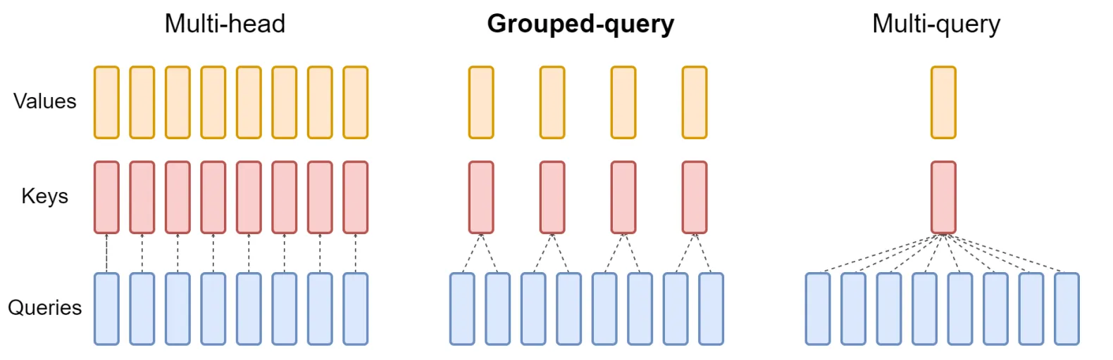
Grouped Query Attention

Grouped Query Attention (GQA) is an efficient variant of multi-head attention that reduces computational cost while maintaining strong performance.

Instead of each query attending to separate key-value heads, GQA groups queries together and shares key-value projections within each group. This reduces memory usage and speeds up inference, making it particularly useful for large-scale models like LLaMA and GPT variants.

GQA strikes a balance between Multi-Query Attention (MQA), which uses a single shared key-value pair, and full Multi-Head Attention (MHA), which has independent key-value pairs for each head. By leveraging grouped keys and values, GQA achieves high efficiency with minimal accuracy loss, making it widely used in modern LLMs for scalable and cost-effective deployment.

1class GroupedQueryAttention(nn.Module):
2    def __init__(self, embed_size, num_heads, num_groups):
3        super(GroupedQueryAttention, self).__init__()
4        self.embed_size = embed_size
5        self.num_heads = num_heads
6        self.num_groups = num_groups
7        self.head_dim = embed_size // num_heads
8        
9        assert num_heads % num_groups == 0, "Number of heads must be divisible by number of groups"
10        
11        self.W_q = nn.Linear(embed_size, embed_size)
12        self.W_kv = nn.Linear(embed_size, embed_size * 2)  # Shared keys and values across groups
13        self.fc_out = nn.Linear(embed_size, embed_size)
14
15    def forward(self, x):
16        batch_size, seq_length, _ = x.shape
17
18        # Compute queries normally
19        Q = self.W_q(x)
20        Q = Q.view(batch_size, seq_length, self.num_heads, self.head_dim).transpose(1, 2)  # (B, heads, L, head_dim)
21
22        # Compute shared keys and values across groups
23        kv = self.W_kv(x)
24        kv = kv.view(batch_size, seq_length, 2, self.num_groups, self.embed_size // self.num_groups)
25        K, V = kv[:, :, 0, :, :], kv[:, :, 1, :, :]
26        
27        # Expand keys and values to match number of heads per group
28        heads_per_group = self.num_heads // self.num_groups
29        K = K.repeat_interleave(heads_per_group, dim=2)
30        V = V.repeat_interleave(heads_per_group, dim=2)
31
32        # Compute attention
33        scores = torch.matmul(Q, K.transpose(-2, -1)) / math.sqrt(self.head_dim)
34        attention = torch.softmax(scores, dim=-1)
35        out = torch.matmul(attention, V)
36
37        # Reshape and project output
38        out = out.transpose(1, 2).contiguous().view(batch_size, seq_length, self.embed_size)
39        return self.fc_out(out)

Explanation

1. Extract batch size and sequence length from input shape

16batch_size, seq_length, _ = x.shape

Retrieves the batch size and sequence length from the input tensor x, ignoring the embedding dimension.

2. Compute queries

19Q = self.W_q(x)

Applies the learnable weight matrix W_q to project x into the query space.

3. Reshape and transpose queries

20Q = Q.view(batch_size, seq_length, self.num_heads, self.head_dim).transpose(1, 2)

Reshapes Q into (batch_size, seq_length, num_heads, head_dim) and transposes to (batch_size, num_heads, seq_length, head_dim).

4. Compute shared keys and values

23kv = self.W_kv(x)

Uses a single linear layer W_kv to compute both key and value matrices simultaneously.

5. Reshape and split keys and values

24kv = kv.view(batch_size, seq_length, 2, self.num_groups, self.embed_size // self.num_groups)

Reshapes the kv tensor into (batch_size, seq_length, 2, num_groups, embed_size // num_groups), separating keys and values into distinct groups.

6. Extract key and value tensors separately

25K, V = kv[:, :, 0, :, :], kv[:, :, 1, :, :]

Extracts the key and value tensors from the reshaped kv tensor.

7. Expand keys to match the number of heads per group

28heads_per_group = self.num_heads // self.num_groups
29K = K.repeat_interleave(heads_per_group, dim=2)

Repeats each key tensor within a group to match the number of heads per group.

30V = V.repeat_interleave(heads_per_group, dim=2)

Repeats each value tensor within a group to match the number of heads per group.

8. Compute attention scores

33scores = torch.matmul(Q, K.transpose(-2, -1)) / math.sqrt(self.head_dim)

Computes the attention scores by taking the dot product of queries and keys, scaled by the square root of the head dimension.

9. Apply softmax to obtain attention weights

34attention = torch.softmax(scores, dim=-1)

Applies the softmax function along the last dimension to obtain attention weights.

10. Combine values with attention weights

35out = torch.matmul(attention, V)

Computes the weighted sum of values using the attention weights.

11. Reshape and project output

38out = out.transpose(1, 2).contiguous().view(batch_size, seq_length, self.embed_size)

Transposes and reshapes the output tensor to match the original embedding size.

12. Final linear transformation

39return self.fc_out(out)

Applies a final linear transformation to the output tensor to mix information across heads.

Applications: Grouped Query Attention is used in models like LLaMA 2 - 70B and Mistral 7B.

5. Infini-Attention

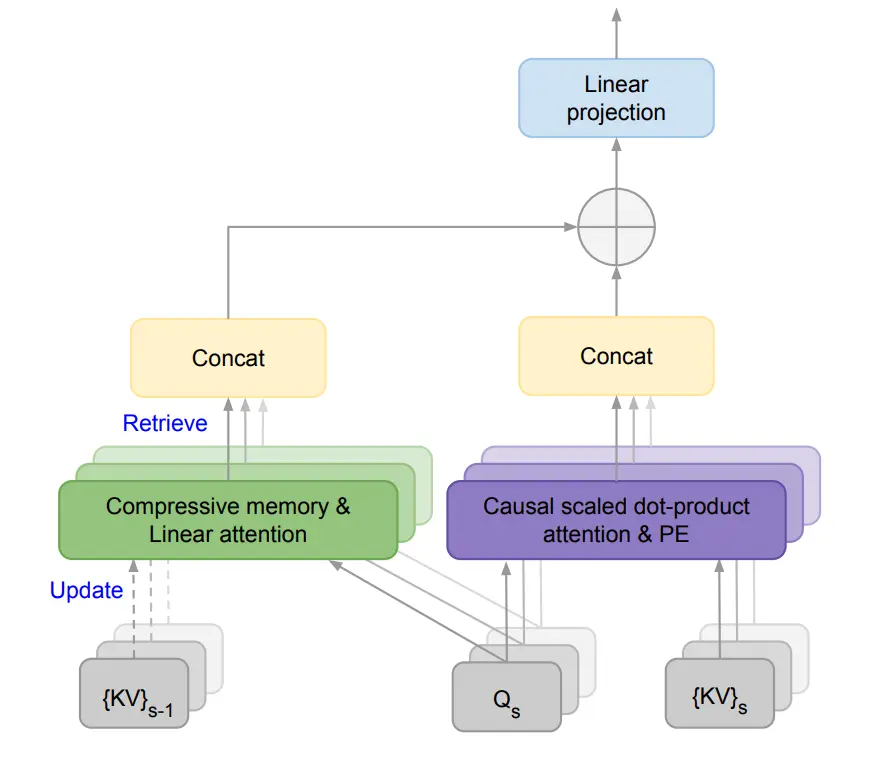
Infini Attention

Infini-Attention tackles the problem of long sequences by processing infinitely long inputs with bounded memory and computation. Think of it as an attention mechanism that can handle a marathon of tokens without breaking a sweat.

This make LLM scalable to very long sequences. But the complexity of design and potential approximations might hurt precision.

Code Example: Infini-Attention Class

1class InfiniAttention(nn.Module):
2    def __init__(self, 
3      seq_len: int,
4      emb_dim: int,
5      d_head: int,
6      n_head: int,
7      n_segments: int,
8      is_causal: Optional[bool] = True,
9      update: Optional[str] = 'linear', 
10      device: Optional[str] = 'cpu',
11      scale:Optional[int] = 10
12    ):
13        super().__init__()
14
15        """
16        Args:
17        seq_len: Sequence length of the inputs.
18        n_segments: Number of segments (must be divisible to seq_len).
19        n_head: Number of attention heads.
20        emb_dim: Embedding dimension of the input.
21        d_head: Embedding dimension of each head.
22        is_causal: Whether the model causal or not.
23        device: cuda or cpu.
24        """
25        if update not in ['linear', 'delta']:
26            raise ValueError('Update takes only one of these parameters - linear, delta')
27        
28        assert seq_len % n_segments == 0, 'seq_len must be divisible to n_segments'
29        assert emb_dim % n_head == 0, 'emb_dim must be divisible to n_head'
30
31        self.seq_len = seq_len
32        self.n_segments = n_segments
33        self.n_head = n_head
34        self.emb_dim = emb_dim
35        self.d_head = d_head
36        self.is_causal = is_causal
37        self.use_rope = use_rope
38        self.update = update
39        self.device = device
40        self.scale = scale
41        self.beta = nn.Parameter(torch.zeros((1,self.n_head,1,1))) # -> A learnable scalar from the paper.
42        self.q = nn.Linear(emb_dim, emb_dim, device=device)
43        self.k = nn.Linear(emb_dim, emb_dim, device=device)
44        self.v = nn.Linear(emb_dim, emb_dim, device=device)
45        self.o = nn.Linear(emb_dim, emb_dim, device=device)
46        self.elu = nn.ELU()
47        self.freq_cis = RoPE.compute_freq_cis(emb_dim, seq_len, 10000.0, device=device)
48        self.register_buffer('causal', torch.tril(torch.ones(seq_len // n_segments, seq_len // n_segments, device=device)))
49
50    def forward(self, x: torch.Tensor) -> torch.Tensor:
51
52        batch_size, _, _ = x.size()
53
54        #There was no guide for initialization for the parameters below, so I just initialize them fron zero.
55        memory = torch.zeros((self.n_head, self.d_head, self.d_head)).to(self.device)
56        z = torch.zeros((self.n_head, self.d_head, 1)).to(self.device)
57
58        query = self.q(x)
59        key = self.k(x)
60        value = self.v(x)
61
62        query = query.view(batch_size, self.n_head, self.n_segments, self.seq_len // self.n_segments, self.d_head)
63        key = key.view(batch_size, self.n_head, self.n_segments, self.seq_len // self.n_segments, self.d_head)
64        value = value.view(batch_size, self.n_head, self.n_segments, self.seq_len // self.n_segments, self.d_head)
65
66        output = []
67
68        for idx in range(self.n_segments):
69
70            sigma_q = self.elu(query[:, :, idx, :, :]) + 1.0
71            sigma_k = self.elu(key[:, :, idx, :, :]) + 1.0
72            A_mem = (sigma_q @ memory) / ((sigma_q @ z) + 1e-6)  # Adding 1e-6 for preventing division to 0
73
74            A_dot = query[:, :, idx, :, :] @ key[:, :, idx, :, :].transpose(-2, -1)
75            
76            if self.is_causal:
77              A_dot.masked_fill_(self.causal == 0, float('-inf'))
78
79            A_dot = F.softmax(A_dot / torch.sqrt(torch.tensor(self.d_head)), dim = -1)
80            A_dot =  A_dot @ value[:, :, idx, :, :]
81
82            attention = (F.sigmoid(self.beta*self.scale) * A_mem) + ((1 - F.sigmoid(self.beta*self.scale)) * A_dot)
83
84            #Update
85            if self.update == 'linear':
86                memory = memory + (sigma_k.transpose(-2, -1) @ value[:, :, idx, :, :])
87            else:
88                delta = (sigma_k @ memory) / ((sigma_k @ z) + 1e-6)
89                memory = memory + (sigma_k.transpose(-2, -1) @ (value[:, :, idx, :, :] - delta))
90            
91            z = z + sigma_k.sum(dim = -2, keepdim = True)
92
93            output.append(attention)
94        
95        attention = torch.concat(output, dim = 2).view(batch_size, self.seq_len, self.emb_dim)
96        return self.o(attention)

Credit: https://github.com/vmarinowski/infini-attention

Explanation

Extract batch size:

52batch_size, _, _ = x.size()

Extracts the batch size from the input tensor x.

Initialize memory and update vector:

55memory = torch.zeros((self.n_head, self.d_head, self.d_head)).to(self.device)
56z = torch.zeros((self.n_head, self.d_head, 1)).to(self.device)

Creates tensors memory and z, both initialized to zero.

Compute query, key, and value:

58query = self.q(x)
59key = self.k(x)
60value = self.v(x)

Projects the input x into query, key, and value spaces.

Reshape for multi-head attention:

62query = query.view(batch_size, self.n_head, self.n_segments, self.seq_len // self.n_segments, self.d_head)
63key = key.view(batch_size, self.n_head, self.n_segments, self.seq_len // self.n_segments, self.d_head)
64value = value.view(batch_size, self.n_head, self.n_segments, self.seq_len // self.n_segments, self.d_head)

Splits query, key, and value into multiple attention heads and segments.

Initialize an output list:

66output = []

Creates an empty list to store attention outputs.

Loop over segments:

68for idx in range(self.n_segments):

Iterates over each segment of the input sequence.

Compute sigma_q and sigma_k:

70sigma_q = self.elu(query[:, :, idx, :, :]) + 1.0
71sigma_k = self.elu(key[:, :, idx, :, :]) + 1.0

Applies ELU activation and shifts values to be positive.

Compute A_mem:

72A_mem = (sigma_q @ memory) / ((sigma_q @ z) + 1e-6)

Uses memory to compute attention, normalizing by z to prevent division by zero.

Compute A_dot:

74A_dot = query[:, :, idx, :, :] @ key[:, :, idx, :, :].transpose(-2, -1)

Performs standard dot-product attention.

Apply causal masking:

76if self.is_causal:
77    A_dot.masked_fill_(self.causal == 0, float('-inf'))

Masks out future tokens to ensure causality in the attention mechanism.

Compute softmax:

79A_dot = F.softmax(A_dot / torch.sqrt(torch.tensor(self.d_head)), dim = -1)

Applies softmax to obtain attention weights. Normalizes scores using softmax with scaling.

Compute value-weighted attention scores:

80A_dot =  A_dot @ value[:, :, idx, :, :]

Computes the weighted sum of values using the attention weights.

Compute final attention mix:

82attention = (F.sigmoid(self.beta*self.scale) * A_mem) + ((1 - F.sigmoid(self.beta*self.scale)) * A_dot)

Uses a learnable weight beta to blend memory-based and standard attention.

Update memory:

86if self.update == 'linear':
87    memory = memory + (sigma_k.transpose(-2, -1) @ value[:, :, idx, :, :])
88else:
89    delta = (sigma_k @ memory) / ((sigma_k @ z) + 1e-6)
90    memory = memory + (sigma_k.transpose(-2, -1) @ (value[:, :, idx, :, :] - delta))

Updates memory based on sigma_k and the update rule (linear or delta).

Update z tensor:

91z = z + sigma_k.sum(dim = -2, keepdim = True)

Accumulates sigma_k values for normalization.

Store attention output:

93output.append(attention)

Saves computed attention for this segment.

Concatenate segment outputs:

95attention = torch.concat(output, dim = 2).view(batch_size, self.seq_len, self.emb_dim)

Joins segment-wise outputs into a single sequence.

Apply output projection:

96return self.o(attention)

Projects the attention output to the final embedding dimension.

Although Infini-Attention is a powerful tool for handling long sequences, it's not yet a widely adopted feature in mainstream LLMs. The complexity of the design and potential approximations may hinder its widespread use. However, as the demand for processing longer sequences grows, Infini-Attention could become a key component in future models.

6. Sliding Window Attention

Sliding Window Attention

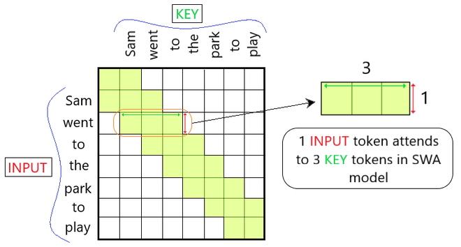
Sliding Window or Local Attention restricts each token’s view to a fixed window. It’s like a gossip session where you only hear what’s happening in your immediate vicinity—not the entire neighborhood.

This method reduces the computational complexity of attention by limiting the interactions between tokens. By focusing on local context, it can efficiently handle long sequences without sacrificing performance.

Coding Example: Sliding Window Attention Class

1class SlidingWindowAttention(nn.Module):
2    def __init__(self, embed_size, window_size):
3        super(SlidingWindowAttention, self).__init__()
4        self.embed_size = embed_size
5        self.window_size = window_size
6        self.W_q = nn.Linear(embed_size, embed_size)
7        self.W_k = nn.Linear(embed_size, embed_size)
8        self.W_v = nn.Linear(embed_size, embed_size)
9    
10    def forward(self, x):
11        batch_size, seq_length, _ = x.shape
12        Q = self.W_q(x)
13        K = self.W_k(x)
14        V = self.W_v(x)
15        outputs = []
16        for i in range(seq_length):
17            start = max(0, i - self.window_size)
18            end = min(seq_length, i + self.window_size + 1)
19            Q_i = Q[:, i:i+1, :]
20            K_window = K[:, start:end, :]
21            V_window = V[:, start:end, :]
22            scores = torch.matmul(Q_i, K_window.transpose(-2, -1)) / math.sqrt(x.size(-1))
23            attention = torch.softmax(scores, dim=-1)
24            outputs.append(torch.matmul(attention, V_window))
25        return torch.cat(outputs, dim=1)

Explanation

1. Extract batch size and sequence length:

11batch_size, seq_length, _ = x.shape

Retrieves the batch size and sequence length from the input tensor x.

Compute queries, keys, and values:

12Q = self.W_q(x)
13K = self.W_k(x)
14V = self.W_v(x)

Projects the input x into query, key, and value spaces.

Initialize an output list:

15outputs = []

Creates an empty list to store attention outputs.

Loop over tokens:

16for i in range(seq_length):

Iterates over each token in the input sequence.

Compute window boundaries:

17start = max(0, i - self.window_size)
18end = min(seq_length, i + self.window_size + 1)

Determines the start and end positions of the window centered around the current token.

Extract query and window keys/values:

19Q_i = Q[:, i:i+1, :]

Extracts the query tensor for the current token.

20K_window = K[:, start:end, :]
21V_window = V[:, start:end, :]

Extracts the key and value tensors for the window around the current token.

Compute attention scores:

22scores = torch.matmul(Q_i, K_window.transpose(-2, -1)) / math.sqrt(x.size(-1))

Computes the attention scores between the query and key tensors for the window.

Apply softmax to obtain attention weights:

23attention = torch.softmax(scores, dim=-1)

Normalizes the attention scores using the softmax function along the last dimension.

Combine values with attention weights:

24outputs.append(torch.matmul(attention, V_window)

Computes the weighted sum of values using the attention weights for the window.

Concatenate attention outputs:

25return torch.cat(outputs, dim=1)

Joins the attention outputs for all tokens into a single tensor.

Sliding Window Attention is a popular choice for handling long sequences in models like Mistral 7B, Longformer.

7. Flash Attention

Flash Attention

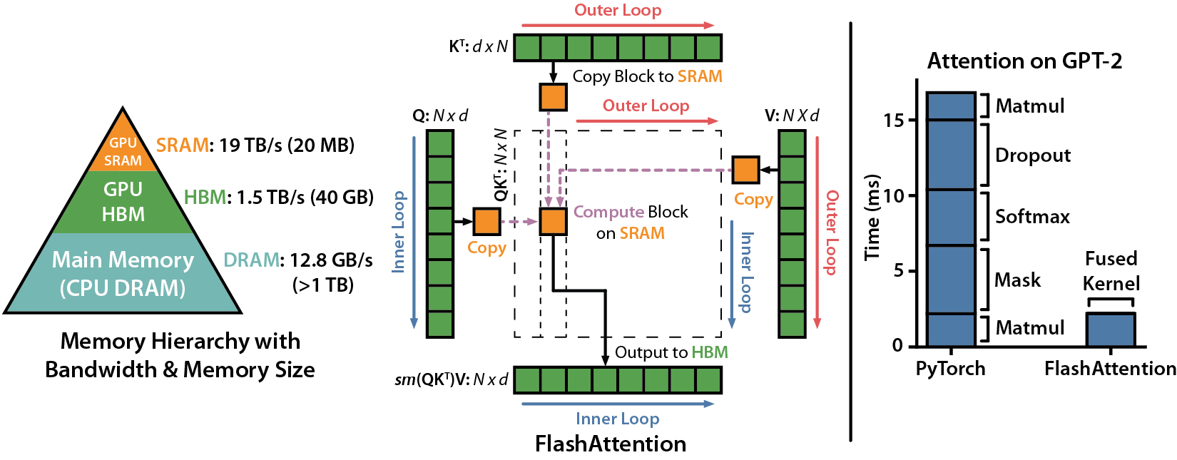
Flash Attention is a performance-oriented reimplementation of vanilla attention. It leverages efficient memory layouts and GPU-friendly operations to calculate attention with minimal overhead. In short, it’s the speedster of the attention family—designed to give you all the power of vanilla attention but at lightning speed.

Flash Attention (and it's versions 2 and 3) are mathematically the same as vanilla attention, but implemented efficiently to reduce memory and speed up computations on GPUs.

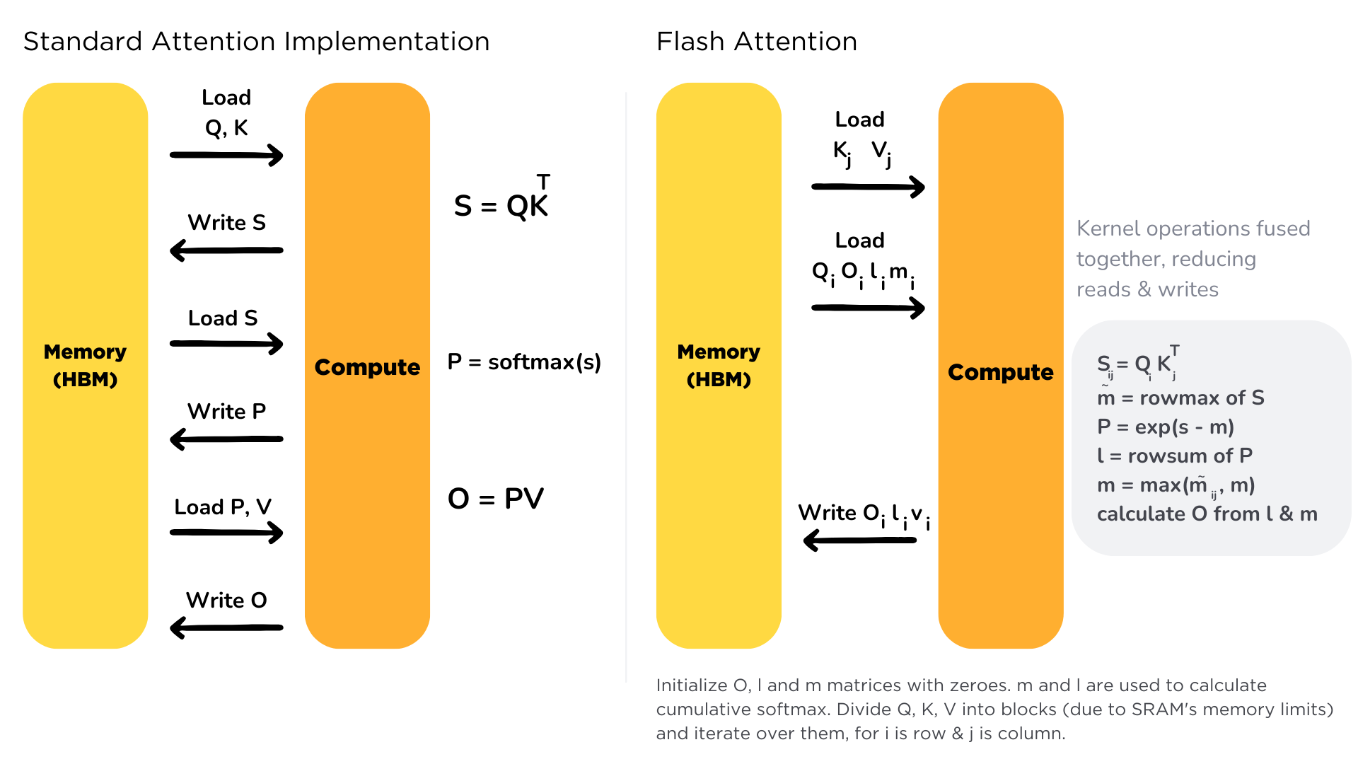
Flash Attention explained in HuggingFace Documentation

Flash Attention Illustration in HuggingFace Documentation

Standard attention mechanism uses High Bandwidth Memory (HBM) to store, read and write keys, queries and values. HBM is large in memory, but slow in processing, meanwhile SRAM is smaller in memory, but faster in operations.

In the standard attention implementation, the cost of loading and writing keys, queries, and values from HBM is high. It loads keys, queries, and values from HBM to GPU on-chip SRAM, performs a single step of the attention mechanism, writes it back to HBM, and repeats this for every single attention step. Instead, Flash Attention loads keys, queries, and values once, fuses the operations of the attention mechanism, and writes them back.

It uses vanilla attention, but with optimizations like:

Kernel Fusion: It fuses multiple operations (matrix multiplications, softmax, and scaling) into a single optimized GPU kernel, reducing unnecessary memory access.
Tiling: Flash Attention divides the attention matrices into smaller blocks (tiles) to optimize memory access and computation efficiency. This allows processing the input in smaller, manageable chunks, reducing the need to store the entire attention matrix in memory.
Recomputation: Instead of storing intermediate results, Flash Attention recomputes them as needed, minimizing memory consumption.
Memory Efficiency: By processing in blocks and recomputing, Flash Attention reduces memory usage from quadratic to linear with respect to sequence length, making it suitable for long sequences.
Numerical Stability: Flash Attention employs techniques like the "max trick" to maintain numerical stability during the softmax computation, ensuring accurate results even with large inputs.
IO Complexity: Flash Attention is designed to minimize the number of accesses to GPU high bandwidth memory (HBM), making it an efficient choice for various GPU sizes.

I would like to include flash attention code over here. But then I realized that it is too long to include. So I will just include the link to the code.
Flash Attention Official Repository

Flash Attention being an efficient reimplementation of vanilla attention, it's widely used in models like Mistral 7B, LlaMA 2 - 70B.

HuggingFace's Transformers library also has an attribute to enable Flash Attention. If a model supports Flash Attention attn_implementation="flash_attention_2".

Conclusion

Phew that was a bit too much, I know! But I hope you enjoyed the journey through the world of attention mechanisms. From vanilla attention to Flash Attention, we've covered a wide range of attention variants that power modern deep learning models.

Attention mechanisms are the backbone of modern deep learning models, enabling them to capture complex relationships in data. By understanding the inner workings of attention, you can appreciate the nuances of different attention mechanisms and their impact on model performance.

Whether you're building a new model or fine-tuning an existing one, choosing the right attention mechanism can significantly affect the efficiency and effectiveness of your model. Each attention variant has its strengths and weaknesses, making it crucial to select the one that best suits your use case.

If you're interested in learning more about attention mechanisms and their applications, check out the following resources:

Attention Is All You Need explained by Yannic Kilcher - Video
The Illustrated Transformer by Jay Alammar - Blog
Attention in transformers, step by step by 3Blue1Brown - Video
Variants of Multi-head attention: Multi-query (MQA) and Grouped-query attention (GQA) - Video
Sliding Window Attention Explained - Blog
Flash Attention explained by Umar Jamil - Video

See you in the next blog! Until then, keep learning and exploring the fascinating world of deep learning.

If this resonated, pass it along.

Share on X ›Share on LinkedIn ›Submit to HN ›

All content licensed under CC BY-SA 4.0 unless otherwise noted.